
This is installment 2 on the question: Is inconsistency a starting-pitcher virtue?
I’m sure everyone read installment 1. But remember, the idea is that holding mean runs allowed constant, a pitcher who pitches brilliantly a good deal of the time but occasionally implodes gives his team more chances to win than one who consistently grinds out middling, or maybe even better than that, performances:

This is the motivating insight of Brill & Wyner, who propose an alternative WAR metric that, unlike FanGraphs’s and Baseball Reference’s, recognizes that variance in runs allowed should be taken into account (positively, if it is high) in ranking starting pitchers.

Last time I presented results of a simulation that tried to figure out whether there is extra value, and how much, associated with higher-than-normal variance in runs allowed. Although it was counterfactual, it tried to be as realistic as possible, simulating games on an empirically derived matching of mean runs allowed to their observed variance distributions.
It found that, yes, higher variance in runs allowed per game—generally, not necessarily by starters—is associated with more wins than you’d expect against a Pythagorean Expectation baseline.
But it also found the effect was concentrated largely in very weak teams—ones with bad pitching and anemic hitting generally—and in any case was very small. Indeed, I ventured the conjecture that it was likely too small an effect to be confidently measured in real-world performances.
Laying out the evidence for that conclusion is the aim of this installment.
It consists of a test with historical data.
What I did was quantify the starter variance of teams’ pitchers, measured in how much their performances across starts deviated from their per-inning expected runs allowed totals.
I measured how such variance affected teams’ winning percentages relative to their Pythagorean Expectation (PE), which views all runs allowed equally without regard to how consistently or erratically they are allowed across games.
I used two PE benchmarks.
The first was a 20,000-replicate Monte Carlo simulation that replayed the seasons of every AL/NL team since 1900. In the replay, runs scored and allowed per game were drawn from empirically grounded distributions centered on their historical season means but with variances equal to the median season ones for teams that score or allow that many runs per game on average. (The methods for constructing these distributions were the same one used in the simulation, and featured a statistical technique called “exponentially tilted empirical likelihood.”)
This “empirical null,” then, gives us a sense of the random distribution of outcomes a team with the same offensive and defensive capacity as any historically observed one would do if its starters were right smack in the middle of the actual variance distribution.
Recognizing, too, that run-scoring dynamics have changed a lot across MLB history, I included in the model variables to measure how playing in any of 7 distinct “run scoring” eras might have affected the impact of starter variance.
Then we can compare to see if historical teams that featured higher-than-normal starter variance won more games than their simulated, variance-neutral/neutered counterparts.
So that was one test—call it MCEN for Monte Carlo Empirical Null.
The other test can be called PEN—for permutation empirical null.
In this one, I randomly permuted the residuals of a model that predicted winning percentage based on their PE-predicted record and their starter variances. Those residuals are the differences between historical teams’ actual winning percentages and the model prediction. The B&W thesis says that teams with higher-variance starters should have lower residuals than ones that don’t: that element of team performance will be capturing an influence on team winning percentage that runs allowed by itself, the only thing PE cares about, is insensitive to.
When the residuals end up shuffled across teams (ones that played in the same season), that completely randomizes the relationship between those residuals and team starter variance. So that furnishes us with another empirical null baseline against which to measure the impact of starter variance on the performance of historical teams. If variance matters, then the historical teams will have much smaller residuals than do their counterparts in the sample in which the residuals were permuted.
These procedures are described in much greater detail in my paper “Against Pythagorean Benchmarking.” That paper uses both MCEN and PEN to test a host of influences that are said to generate deviations in teams’ records relative to their Pythagorean Expectation.
It finds that none of them actually do.
And that includes starter pitcher variance:
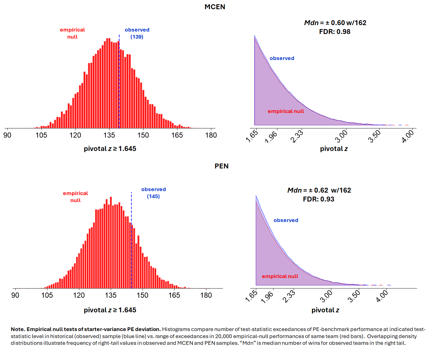
What these figures do is simply count how often a historical team experiences a starter-variance-correlated deviation from its Pythagorean Expectation winning percentage, on the one hand, and how often its counterparts in the MCEN and PEN samples do, on the other.
Because MCEN and PEN were deliberately constructed in a manner that breaks the connection between deviating from PE and starter variance, every team that appears to do so in those samples necessarily did so as a result of chance alone. For us to infer that starter variance generates non-chance PE deviations in the real world, then, the historical teams would have to deviate much more often than the ones in the empirical null samples.
But as you can see, they didn’t. In both MCEN and PEN, historical teams deviated at essentially the same rate as their empirical-null, variance-neutered doppelgangers.
We can quantify the practical import of this finding with a False Discovery Rate (FDR) test.
The FDR uses the ratio of “significant” deviations in the empirical null and historical samples to determine the probability that any observed “statistically significant” relationship of interest—here between starter variance and an historical team’s deviation from PE—is a “false positive,” a fake that is really something consistent with chance alone.
In this case, the FDR was 0.98 for the MCEN test and 0.93 for the PEN test. You can think FDR as a “false positive rate”: it tells us what the probability is that an observed-sample team that meets the test-statistic threshold did so as a matter of chance. (The overlapping density distributions visually illustrate: for MCEN, the ratio of the overlapping region is about 49 times as large, and for PEN 13 times, as the blue observed portion of observed sample teams in the z ≥ 1.645 tail.)
The Figures also note the median number of wins (or losses) per 162 games by which teams that satisfied the threshold deviated from their Pythagorean Expecatation. The size of those effects is quite small, then–around 0.6 wins per 162 games. And if we pick out any one of the 140-odd teams that have have done that over the course of AL/NL history, the odd are between 13:1 and 49:1 that it did so by chance.
Or not really being all that enamored of “statistical significance,” I’d just say that these analyses imply the high-variance effect, however “real,” is just too small to be confidently detected, and hence too ephemeral to be credited in any sort of practical decision or appraisal.
This result, then, reinforces the conclusion of the simulation.
But this is just one evidence-based attempt to answer a really interesting question. I’d be thrilled to see what others—including B&W—found in tests of their own.
My conclusions are always works in progress! Or as Yogi Berra might have put it, there are no singing fat ladies in the empirical Bayes study of baseball.