
So I’ve been knocking myself out for about 3 months revising & reworking a paper on Pythagorean Expectation Benchmarking—or PEB.
PEB is the use of teams’ Pythagorean Expectation (PE) winning percentage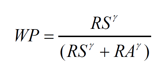
as a benchmark or baseline for assessing the impact of one or another element of team composition.

Commentators have used PEB to advance that claim that all kinds of things—from manager acumen to bench depth to relief pitching to starter variance—are of consequence to teams’ records.
No doubt many of these (if not all of them) are consequential.
But for that to be established by PEB, these elements of team composition have to be shown to add (or subtract) wins over and above the influence they have on team runs scored and allowed. That has to be shown because PE predicts team winning percentage based on just that—runs scored and allowed. So if something is identified as causing teams to be over- or underperforming their PE winning percentages, that team characteristic must be having some effect on team records that a simple tally of team runs scored and allowed misses.
At this point, I just don’t believe any such claim can be established. If you want to see an extended account of why—replete with lots of data—then you can read my working paper “Against Pythagorean Benchmarking.”
But if you want to see a (relatively) more compact account—well, read on! I’m going to compress everything you need to know down to three points.
The two “nonordinary variance channels” of PE deviation
It’s really obvious, but in order for teams to have winning records, they must score more runs than they allow.
What makes PE such a super strong predictor of team winning percentages (90% of variance explained) is that its terms (particularly the magic exponent, γ) encapsulate the effect of how baseball teams’ runs get spread out—their variance—across games.
In any sport, if one knows how much scoring a team generates and yields per contest on average, and how such scoring per game varies in that sport generally, then one can use PE to predict very accurately what that team’s winning percentage is likely to be.
Thus, for a team to deviate from such a prediction, it has to either score or be scored upon in a manner that defies that ordinary level of variance.
Consider run scoring in baseball.
Imagine a season in which a team’s runs scored per game (RSG) variance was lower than ordinary. In that season, it is more likely to have exceeded its PE winning percentage: necessarily, a greater than expected share of its runs will have occurred in close-scoring contests, when those runs were in fact most valuable, as opposed to games in which the team was already comfortably ahead.
In contrast, in a season in which the team’s RSG variance was higher than ordinary, it is more likely to have fallen short of its PE-projected record: in that situation, it will appear, at least, as if the team “wasted” in blowouts runs that it could more profitably have used to change the outcomes of games lost by narrow margins.
The mirror-image effects occur for runs allowed. If a team’s runs-allowed per game (RAG) variance was lower than ordinary in a particular season, it is more likely to have underperformed relative to PE: now the team’s opponents will be the ones to have scored disproportionately when runs mattered most, namely, in close games. On the other hand, after a season in which the team’s RAG variance was higher than ordinary, it is more likely to have overperformed relative to PE: if more than the expected number of runs the team allowed occurred in games in which it was being blown out, then necessarily a greater than ordinary proportion of its opponents’ runs were harmless—crossing the plate in contests that were already “lost causes” from the team’s point of view.
So let’s call these the “nonordinary RSG variance” and “nonordinary RAG variance” channels of PE deviation—or Channel 1 and Channel 2—respectively.
Nonordinary variance just doesn’t matter very much!
Now that we have identified the two PE deviation channels, we can investigate just how much of a difference progressing down one or another makes.
The answer: not much at all!
As explained in more detail in the paper, I constructed a realistic simulation model to get at this.
The guts of it comprise an empirical mapping of varying RSG/RAG means and the distribution of corresponding RSG/RAG variance levels. With that mapping in hand, we can replay as many seasons as we like in which we assign a team whatever mean RSG or RAG we like at whatever point in the associated variance distribution we desire.
You want to know how a team that scores a low, high, or medium number of runs per game will do when its RSG variance is lower or higher than ordinary? Or how a team that allows a high number of runs per game will do when its RAG variance is relatively low or high?
Well, we’ll simulate a 162-game season for it and find out.
Moreover, we can perform this analysis at whatever period of baseball history you are interested in: the data that drives the simulator is aware of how the RSG means/variance relationship has shifted over baseball history.
Consider:
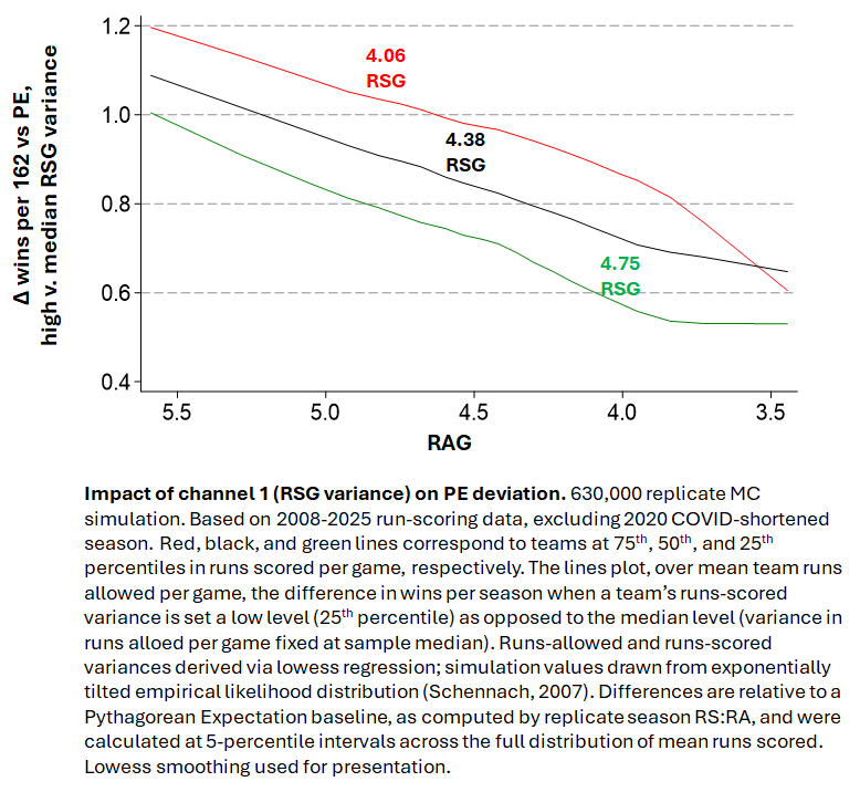
This Figure examines the Channel 1 effect—nonordinary RSG variance—influences team records. It is based on 2008-2025 AL/NL seasons.
The Figure traces how the difference between having low RSG variance (25th percentile) and median RSG variance affects the records of teams of different offensive strength (25th, 50th, and 75th) percentile. The effects, moreover, are plotted in relation to their run-suppressing capacity—i.e., how many runs allowed per game they allowed on average.
We see that RSG variance matters in exactly the way Channel 1 says: lower variance in RSG predicts more wins per season relative to the teams’ PE-predicted winning percentage.
But look at how tiny the effect is! Low RSG variance matters most for teams that simultaneously display the weakest defenses and offenses, and even then the effect is barely over 1 win per season more than PE predicts! The effects, moreover, are much smaller for teams that score more or allow fewer runs per game on average.
Do you really think any practical decisionmaking can be made on the basis of a feature of team composition (manager acumen, say, or relief-pitcher effectiveness) that matters so little and varies so much based on even more basic elements of team quality?
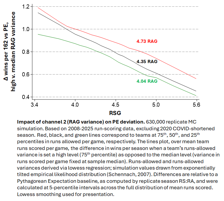
The second plot examines the effect of Channel 2—RAG variance—on PE deviation.
The story is pretty much identical. Teams that have high RAG variance exceed their PE expectation—just as expected—but by a teeny tiny amount (around 1 win a season) and only when are below par in both offensive and defensive capacities.
As teams become less awful in scoring and preventing runs, highRAG variance predicts less and less deviation from their PE-predicted wins per season.
Again, no practical decisionmaker—say a GM constructing a team roster—is going to bother with a factor this tiny and this conditional on other aspects of team performance that matter so much more.
The kicker: these effects are not statistically detectable anyway
The empirically realistic simulation results just presented are ideal, measurement-error free estimations of the impact of Channel 1 and Channel 2 PE deviations.
But in the world, there’s no error-free lunch. PE itself is only a model—and thus subject to sampling error. Likewise for all the estimates based on the empirical RSG/RAG means and variances that drive the realistic simulation model.
To be statistically observable, the (modest) signal that passes through PE-deviation Channels 1 2 have to be loud enough to be heard above of the noise associated with these model components.
Turns out we can estimate how big PE-deviation effects have to be in order to do that.
Exactly how is spelled out in more detail in “Against Pythagorean Benchmarking.” But the basic ideas is simple: using an empirical null, we can simulate how big an impact any asserted influence on PE deviation (manager acumen, reliever effectiveness, starter variance, etc.) would have to be to generate an effect consequential enough for us to take seriously.
In the paper, I do such an analysis using two convergent empirical-null baselines.
The analyses show that the impact would have to be big enough to generate a PE deviation of 2.8 wins (or losses) per 162 games for every standard deviation change in the quality of the putative PE-deviation influence.
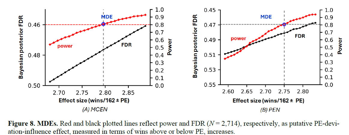
Because PE already explains so much variation in team winning percentages, a “minimum detectable effect” or MDE of 2.8/162 is actually a lot.
It would effectively have to increase the 90% variance explained by PE to around 95%.
 No one who studies the effect sizes of baseball performance metrics is going to believe that such an effect—one that would nearly extinguish all the variance there is to explain in the records of Major League Baseball teams—is achievable.
And in any case, this level of effect far exceeds the very modest Channel 1 and Channel 2 effects that we have reason to believe could possibly be occurring, given the empirically realistic simulation results.
So there you go!
First, we know what’s going on—nonordinary RAG and RSG variances are occurring—when PE deviations are observed.
Second, we know that when we look at the estimated impact of such variances, they are tiny.
And finally, we know that the tools that statics supplies for measuring PE-deviation effects are not sensitive enough to confidently detect ones of that magnitude anyway.
Now, this doesn’t by any means imply that we can’t measure what aspects of team composition make teams more likely to win or lose baseball games.
It means only that PEB is a flawed strategy for doing so. The impacts that matter are the ones that cause teams to score or avoid more runs—and those are all already accounted for in any team’s PE-expected winning percentage.
If we want to use analytics to help identify sources of variance in team performance, then, we need to move upstream of PE—to the point at which we can generate greater insight into the elements of team performance that generate the outputs—runs scored, runs averted—that PE operates on.
And that’s all you need to know about PE Benchmarking.
Or if you want an even more succinct account of what you need to know: just don’t do it!