Strat-o-Matic-playing monkeys go to mWAR (measuring managers part 4)

update 1.9.26: To see the paper that reports the results of the manager estimator into which mWAR evolved (much as we did from chimpanzees), click here.

Okay, let’s continue our examination of manager WAR or MWAR.

As explained last time, MWAR is a career-level measure of manager-value added to (or subtracted from) team performance. It’s measured, appropriately, in relation to the expected wins associated with the aggregate WAR of a managed team’s players. Although measured in relation to the impact of an average manager of a .500 team, MWAR can still fairly be characterized as quantifying a manager’s value over a “replacement” if you accept (as I imagine you would on reflection) that there are an ample supply of unemployed prospective managers (former ones, minor league ones, reflective former players, strat-o-matic junkies etc.) who could guide a team as well as an “average” manager would.

We have been using MWAR to determine how many “extra wins” per season–MWAR_162—can be credited to managers with ≥ 1,000 games managed.

Now it’s time to put MWAR to the monkey test. As we did to appraise Horowitz’s PH, we will conduct a Monte Carlo simulation in which we replay (1,000 times each) the seasons of our manager’s teams, this time using their team WARs to predict their records. Each team will be managed by a monkey-manager counterpart of one of our real-world managers. We’ll examine the MWARs our monkey managers acquire over 131,000 careers to determine what sort MWARs a collection of utterly skilless managers could acquire by sheer chance (again, we’ve selected monkeys with no prior baseball knowledge for this experiment).

What statisticians refer to as an “empirical null,” the MWAR distribution associated with our MC-MPS—“Monte Carlo Monkeys Playing Strat-o-Matic”—simulation can then be used to interrogate our observed, human MWAR distribution. The juxtaposition of the two distributions will help us to figure out when we should regard human managers’ MWAR_162s as true measures of their impact on game outcomes.

We’ll follow the same steps we followed to test Horowitz’s PH.

First, we’ll eyeball the MC-MPS empirical null distribution in relation to a normal, “theoretical null” one. That helps us figure out what real randomness looks like for MWAR.

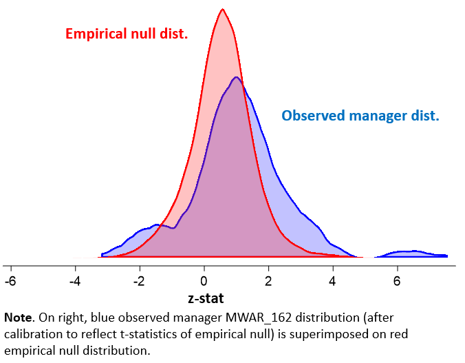
Second, we’ll eyeball how the our real-world MWAR distribution compares to the monkey empirical null. The shape will give us a clue whether we have true difference-makers among our featured human managers.

Third, we’ll perform some Bayesian testing aimed at forming concrete probability estimates of our managers’ impact on their teams’ records.

Ready?

First, here is the MWAR empirical null—the monkey manager WAR distribution—superimposed on a “normal distribution.” Actually, the distributions aren’t MWARs, which we defined in last post as a manager’s career “wins added,” but rather z-statistics of marginal winning percentages relative to a .500 team (the latter determines both the MWAR and MWAR_162 distributions in a straightforward linear fashion).

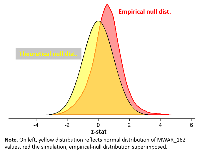
What we see is that the empirical null is definitely more dispersed—spread out—than a normal distribution. That means that it’s even more likely than a conventional (frequentist) statistical analysis would suggest that the performances of managers who appear to have large positive or negative MWAR_162s are indistinguishable from those skilless monkeys. Or in other words, even some seemingly “statistically significant” MWAR_162s are likely a product of chance.

But second, take a look at the observed, human manager distribution relative to the empirical, monkey-manager null one. See that tail puffing out on the right? It belongs to the human managers, not the monkeys! And it signifies that many of them did achieve impacts (successful ones) that one wouldn’t see by chance!

Third, through the magic of empirical Bayesianism, we can now compute new MWAR_162s that reflect revised estimations given the evidence.  

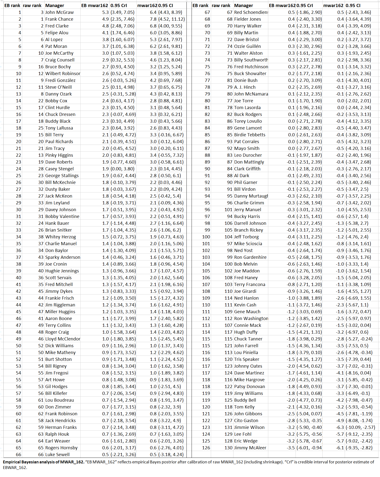Some things to note include:

1. The top-end estimates are lower, and bottom higher (not as far below 0), than the raw model estimates reported last time. That’s a result of “shrinkage,” the property of Bayesian estimates to “shrink” values toward the global mean (here 0).
2. There were some shifts in rankings! Now John McGraw is our new leader, e.g! This can happen, too, as a result of Bayesian analysis. The combination of recalibration and shrinkage can shift the rank order of raw model estimates depending on the precision, or error, of those estimates.
3. Whereas the model estimates had 0.95 “confidence intervals,” the new estimates have Bayesian “credible intervals.” The former tell us what values are < 5% to be observed if we assume the “null”—that no manager has any real impact. The model doesn’t have any idea what the true manager impact might be; and even if we were now to assume the null is “false” with respect to particular managers, the model wouldn’t be telling us what the manager’s actual MWAR_162 is or how confident we should be about that estimate as opposed to others. Those are things we can learn from a Bayesian estimate. The Bayesian estimate has the necessary elements (principally priors and likelihoods — absent from a frequentist, null-hypothesis test) to generate a range of values and associated probabilities for true MWAR_162 of any manager! The mean value is the most probable true MWAR_162; but to know how much more probable it is than another one, we’d have to see the shape of the distribution of the entire range.  The “credible interval” is based on that: it says that we should be 95% confident that the true value of the manager’s MWAR_162 lies within the indicated range.

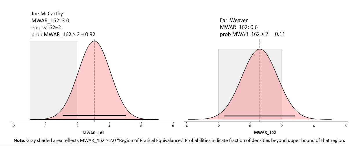
With this sort of information we can now calculate the probability that the manager’s “true” MWAR_162 exceeds a specified threshold.  We did this same sort of thing with Horowitz’s PH, you might recall.

Imagine we want to figure out the probability that a manager’s actual MWAR_162 exceeds 2 games.  Maybe we think that anything less than that is “practically equivalent” to 0 (in which case, ± 2 wins is our ROPE, or “region of practical significance”), or maybe we just think it would be interesting to figure out that out.  Consider:

We can also do crazy things like estimate the probability that,  oh, Felipe Alou generated at least 1.5 wins more per season than Sparky Anderson:

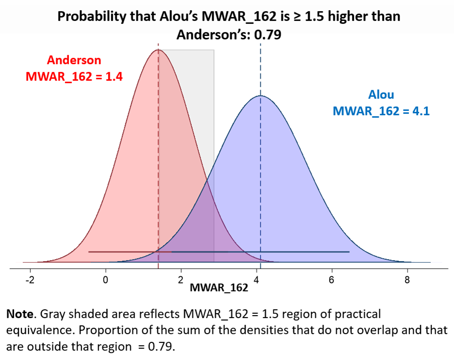
Do you believe this?

Well, you should, I think, believe that these conclusions are true about “MAR_162s.”  I’ve shown you that MWAR ratings are not just a matter of chance and yield, with the benefit of valid statistical techniques, probabilistic estimates of the quantities being measured.

So the estimator is measuring something, and doing so in an admirably precise and reliable way.

But, again, that’s different from external validity: the correspondence between what an estimator is measuring and the real-world phenomenon we are interested in!

It’s hard to externally validate a model of managerial value. We can’t compare the results of the estimator to “real thing” because managerial quality, even assuming it exists, is not directly observable.

The best we can do, I think, is try to develop several internally valid measures that we have good, practical reason to believe should be measuring what we care about, and compare their results. If they agree, then we have all the more reason to believe the validity of each one.

Well, so far we’ve tested two manager-value estimators: Horowitz’s PH and MWAR.  Do they converge to a degree that should give us confidence in their external validity?

I don’t think so.

For one thing, look at the disparities in the models’ respective rankings of top managers. The unlikely run-away PH champ was Aaron Boone; he’s ranked 46 of 131 under MWAR.

By the same token, John McGraw, the MWAR champ, finished with a zero-impact PH = 1.0.

Earl Weaver, third on the PH all-time best list, for example, ended up pretty much right in the middle of the pack in MWAR.

But the two systems are not totally devoid of agreement (sorry, Buddy Bell). Indeed they are correlated 0.45, which suggests that they are at least getting some shared piece of an unobserved quality in the featured managers, even if not a huge shared piece.

Still, I can’t at this point say that I feel very confident in these measures.

We’re going to have to find at least one more!