
 Hey—you remember Mr. BLUP, right? Also known as the “best linear unbiased predictor,” Mr. BLUP supplied a cool benchmark in our study of the performance of park-factor adjusted estimators of “true” or latent batter skill.
Well now Mr. BLUP has graciously agreed to take time off from his day job (evaluating the innate breeding potential of cows) to help with our construction of a manger-value estimator!
As you’ll no doubt recall, we’ve examined two candidate estimators so far: Horowitz’s PH and mWAR. Testing them with our MCMPS—“Monte Carlo monkeys playing Strat-o-Matic”—simulator, we learned that each identified a decent number of managers from our 131-member sample (comprising all the guys who’ve managed ≥ 1,000 MLB games) as having affected the winning percentages of their teams by at least 1.5%. Some affected it positively, others negatively!
The trouble was that the estimators’ conclusions about who these managers were wasn’t super consistent. Their evaluations were not wholly unrelated (r = 0.45), but it was still annoying that Aaron Boone weaseled his way to the top of Horowitz’s PH but was buried in the middle of the pack by mWAR.
This is bothersome not because we care where Aaron Boone ends up but because consistency is critical for this sort of project.
As I’ve explained, the sort of tests that we’ve been doing are aimed at internal validity: they can help show that the estimators we’re evaluating are measuring something reasonably well.
But how do we know they are really measuring what we care about—manager value?
Externally validating the estimators is really hard because manager value isn’t directly observable. It isn’t even attended by accessible indicators of latent ability—like OPS, say, and FIP, which we know are good for estimating innate batter and pitcher skill because they correlate so well with runs (produced by the former and stifled by the latter).
In this situation, pretty much the only thing we can do is find a variety of independent, internally valid estimators that we have good, practical reason to believe line up with manager performance–and then hope they agree. The idea is that it’s less likely that a group of independent estimators would somehow manage to agree with each other if they were all measuring the wrong thing than it is that they’d agree if they were measuring the right one! This is a convergent validation strategy.
Because Horwotiz’s PH and mWAR agreed only modestly, we are trying (desperately) to find at least one more manager-value estimator. If we are lucky, the triangulation of them will then give us reason to think we are zeroing in our target.
Which bring us to . . . Manager BLUP, or mBLUP, for short.
BLUPs are just the random intercept in a multilevel model. When those intercepts are individuals engaged in some task, BLUPS can be conceptualized as capturing some otherwise unmeasured, innate differences that are being obscured by (or at least conflated with) observable differences in the individuals’ situations.
This strategy has worked superbly in animal science, the native domain of BLUP, where random-intercepts enable the qualities that influence the breeding quality of livestock to be separated from the impacts of climate, feed, the music farmers use to get horses and sheep in the mood, and so on.
So why shouldn’t BLUPs help us to part the curtain of confounding variables conspiring to obstruct our view of true manager skill? Well?! Well???!!
That curtain consists principally in the skill of players, of course. A valid estimator must abstract from team quality in order to isolate the manager’s contribution to a team’s won-loss record.
So in our multi-level model, the fixed effects were OPS, FIP, and a composite of the best measures of fielding proficiency. Together these explain about 80% of the variance in team winning percentages—a tad higher than WAR. Based on the models we’ve fit so far, I’d guess that manager differences explain at best 20% of the remainder—meaning just under 2% overall.
That’s not a lot but it could certainly be 2 or 2.5 extra wins—or losses—a year. That’s why I’ve been focusing on ± 1.5% impact on winning-pct as a threshold for treating a manager’s effect as a meaningful one.
In the studies of mWAR and Horowitz’s PH, we used empirical Bayesianism—animated (as it were) by simulations (the monkey managers playing Strat-o-Matic) that supplied us with realistic, “skill-free” benchmarks for evaluating the model estimates of manager impact.
We can’t do that here. In simulations, monkeys—that is, phantom, information-free random intercepts—tend to shrink to zero.
But we can still use a conventional Bayesian multi-level model. Such a model uses estimation strategies that determine how likely a prior hypothesis is given the observed evidence.
The relevant priors here related to the win-pct effect-size associated with the individual manager random intercept. In effect, I specified two: 0 vs > ± 1.5% marginal impact on winning percentage, after taking account of the player performance fixed effects.
One also has to specify a prior distribution on these hypotheses, since in any attempt to measure them, they will take on a range of possible values as a result of measurement error. I picked a distribution that has slightly fatter tails than a normal one (a “half student-t”). This is a decent fallback when one has only modest knowledge of what the characteristics of the relevant variables are—and is in line with what I’d seen in the previous studies of manager effects.
So what did we—or I should say, Mr. BLUP!—find?
Well, some pretty interesting things.
One was that there’s a non-trivial probability that a decent number of managers have exerted a ± 0.015 win-pct impact! The model (which took four hours of running time to fit on computer with a beastly processor and 16 separate cores) generated information that made it possible to extract quantifiable evidence about that.
Indeed, we could use the model to test and form probabilistic judgments about any number of competing hypotheses relating to the number of such mangers in our 131-member sample. E.g., the probability that the number of difference-makers (positive or negative) is somewhere between, oh, 8 and 20 is 95%.
If we focus only on positive impacts, the model indicates that there is a 94% that the at least 5 managers increased their teams’ winning percentages 1.5% over the course of their careers:
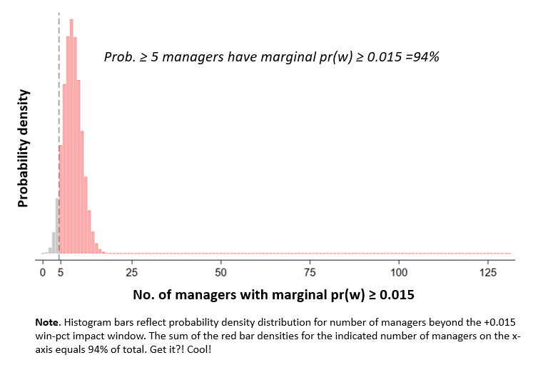
That’s the fraction of the model-generated, probability density distribution (PDD) that includes at least 5 managers who made a 1.5% difference:
By the same logic, the probability that at least 7 managers positively influenced their teams prospects to that degree is over 75%.
That’s interesting, right?
 But here’s another interesting thing: the model doesn’t give us nearly so much information about who those managers are!
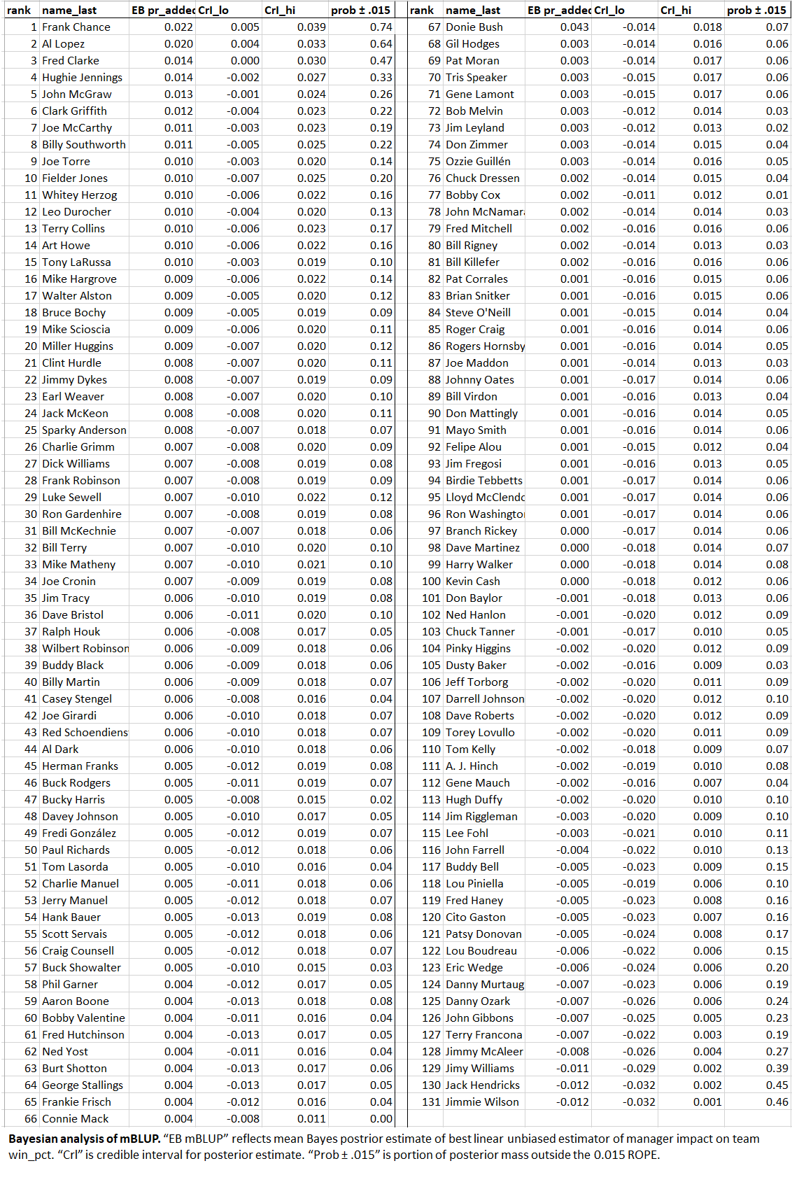
The model indicates that there is a 75% chance Frank Chance had an impact that large. There’s a 64% chance that Al Lopez did.
But those are the only two individual managers for whom the evidence supported a more-likely-than-not probability of crossing the 1.5% impact line!
This isn’t that strange really. The evidence on the individual managers consisted of their season-by-season records; for most that was well under 20. Because we are comparing distributional ranges of values when we look at competing hypotheses from a Bayesian perspective, competing ones will be pretty diffuse and thus tend to overlap a lot when you have so few observations.
For the sample as a whole, though, there were many more: 131x as many as for the average manager. Now we are starting to form a much sharper picture of the boundaries of hypotheses associated outcome ranges.
But none of this means that we didn’t learn anything about our individual managers!
Each one of them has an evidence-derived, probability density distribution of “marginal winning-pct” impacts. Those densities can be compared with each other to make comparative judgments about the likelihood that one manager versus another exceeds the 1.5%-impact threshold!
Consider:
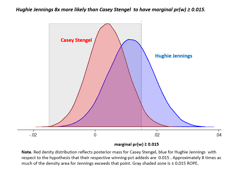
It we just ask, “how much did Hughie Jennings and Casey Stengel influence their teams’ winning percentages,” the most likely answer for both is roughly 1%, or within within my personal “meh” region. But because we are, among other things, trying to value managers relative to each other, we’re learning something when we can say in addition that Hughie Jennings is 8x more likely than Casey Stengel to be one of the 5 or more mangers who we’re 94% confident (or one of the 7 we are 75% confident) had a 1.5% positive impact on his team’s winning prospects!
But let’s be clear about what that means. It doesn’t indicate that there is a 88% (8:1) probability or even a > 50% probability that Jennings improved the Tigers’ winning percentage by ≥ 1.5% during his tenure. (The data say there was a 32% of that.) All it means is that between the two, the evidence is 8.1x more consistent with Jennings being one of the positive difference-makers than with Stengel being one.
This is a Bayesian likelihood ratio (or “Bayes Factor”). It characterizes the weight of the evidence in favor of competing hypotheses.
It doesn’t tell you what the probability is of that hypothesis being true, however. To get that, we need to use the likelihood ratio in conjunction with our prior—that is, our belief about the probability of the hypotheses formed before (or independently of) this new evidence.
Under Bayes’s theorem, we determine how much to adjust the strength of our beliefs according to this relatively straightforward formula:
![]()
Prior odds are what they sound like: the odds you put on a hypothesis before you encounter the new information in question. Posterior odds mean the odds you put on that hypothesis after taking the new information on board. Bridging the two is the likelihood ratio, which is how much more consistent the new evidence is with that hypothesis than with some other, competing one. The likelihood ratio, then, characterizes the weight of the new evidence—with a ratio of 1 being equally consistent; a ratio > 1 more; and a ratio < 1 less consistent than with the alternative.
So say you started out believing that Stengel was 10x or 10:1 more likely than Jennings to be one of the positive difference-makers in the sample. What do you do when I tell you I have validly derived evidence that Jennings is 8x more likely than Stengel to be in that class? Well, multiplying 10:1 (the prior odds in favor of Stengel) by the likelihood ratio of 1:8 (the likelihood of observing this evidence if that hypothesis rather than its negation were true), you should now believe the odds are 10:8 or 5:4 (55%) that Stengel is more likely to be one of the members if the “+ 0.015 club.
 Of course, if you started off with the belief that there was a 3:1 greater chance (75%) that Jennings had such an impact than that Stengel did, you’d now believe the odds in favor of that hypothesis are 24:1 (96%; sounds right!). Either way, keep snooping around for more evidence, and keep updating based on it — baseball science is a permanent procession of conjectures and refutations (I’m pretty sure that it was Casey Stengel who said that).
Hey, I don’t know about you, but I prefer a statistic that tells me how strong the evidence is and lets me decide what to believe over one that just tells me the probability of a fact and insists I believe it!
Bottom line: even if we can’t be sure who the five or more managers we are 94% confident improved their teams’ win pcts by at least 1.5%, we can get a lot of information out of this data to help us assess how strongly the evidence supports competing claims about who they might be!
Thanks, Mr. BLUP—that’s pretty neat! Good luck with your goats and sheep this week!
But now: how far have we progressed toward our ultimate goal—to figure out whether any of the manager-value estimators we’ve looked at, including this one, is externally valid?
Have we reached convergent validity yet?
That’s the $1,000,000 question (a modest amount by today’s standards, I grant).
If you want to know the answer –or at least my shot at an answer; yours might differ—you’ll have to tune in next time!