This is more or less what I said:
My focus is manager value, one of the last aspects of major league baseball unaffected by the sports analytics revolution. The goal of the paper is to fashion a manager-value estimator akin to player WAR—one that can validly quantify the impact of managers in terms of wins or added per season.
The basic analytical strategy is to assess managers in relation to a team-performance models based on player value. If a manager’s teams do systematically better—or worse—than predicted by these benchmark models, we can infer that the manager is responsible for that impact.
The paper examines three candidate benchmarks but I’ll focus here on two: one based on the Pythagorean Expectation formula and another on player WAR. I’ll describe, too, how I used simulations to identify manager impacts.
As everyone knows, the Pythagorean Expectation formula predicts winning percentage on the basis of runs scored and allowed.
How a team fares in relation to its PEF is based entirely on its run-scoring distribution. If a team overperforms its expectation, that implies it had lower run-scoring variance, effectively conserving runs for wins in close games. If a team underperformed, then necessarily it had higher run-scoring variance, wasting in blowouts runs that would have been more profitably used in close contests.
The question, then, is do managers affect variance levels in their teams’ run scoring? Does their strategic decisionmaking result in a sufficient surplus or deficit of close wins to make the team deviate from its PEF-predicted winning percentage?
To test that, I perform a Monte Carlo simulation. Every one of the managers games are replayed with runs scored and against drawn from distributions pegged to their teams’ season means. Bur rather than use the teams’ actual run-scoring variance, we use the league standard deviation for that season.
So teams end up with their average runs scored and allowed but with a level of run-scoring variance necessarily unrelated to manager skill. We do this 10,000 times, using a model in which any team deviation from PEF is assigned to a phantom or monkey manager, who necessarily exerted no impact. We then compare the real-world managers’ records to their monkey manager stand ins.
The same basic strategy is used for the player WAR benchmark. Player WAR explains over 80% of variance in team winning percentages. The question is whether their managers are responsible for any the residual.
Again we can form an answer using a simulation, this time a parametric bootstrap. We first estimate every teams’ record using a player-WAR only model. Then we generate 20,000 seasons based on that model. After that, we refit the player WAR model to those seasons adding monkey manager covariates. Their records are then used as the benchmark to see if their real-world counterparts had more than a random impact on their teams’ records.
These are the distributions of monkey manager records in the simulations. You can see that the expected number of monkeys ended up with either extremely good or extremely bad records relative to the benchmark models. But these monkey manager impacts are counterfeit ones; they arise sheerly by chance.
For real managers to matter, the proportion who have really good or really bad records has to substantially exceed the proportion of monkey managers with such records.
That doesn’t happen under the Pythagorean benchmark. There is a 94% poster4ior probability that any manager who exceeds the z 1.96 threshold is a false non-null.
So either real managers are no more effective than monkeys playing strat-o-matic or the Pythagorean benchmark is not a good one for testing manager value.
I think it’s the latter, for mathematical reasons having to do with the way the Pythagorean formula works.
But this conclusion is fortified by the results under the player WAR benchmark. There we we see that manager impacts far outstrip those of the monkey managers. Apparent impacts beyond the z 1.96 threshold are almost 2.5 x as likely to be genuine than specious.
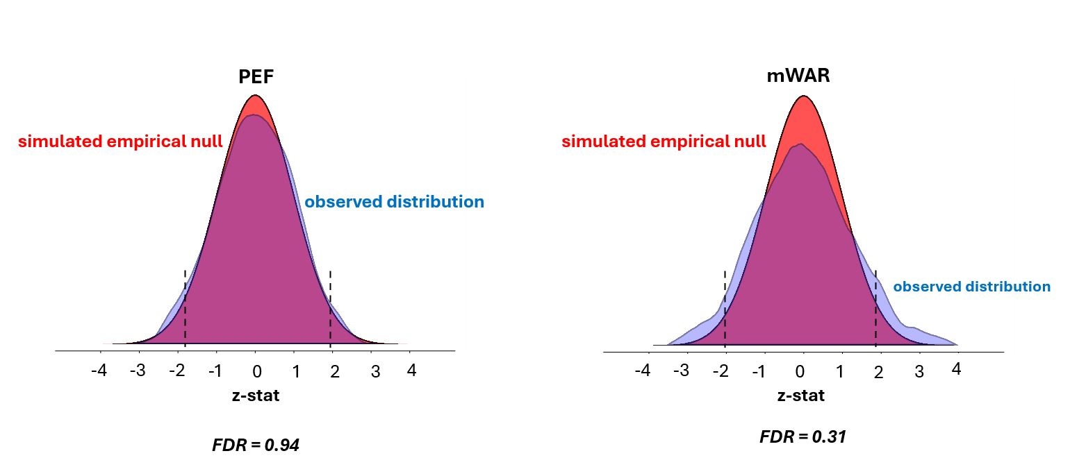
But the goal here isn’t to determine whether manager impacts are “statistically significant”; it is to quantify any genuine impact the simulations show exists.
For this, Bayesian statistics furnish the best tool.
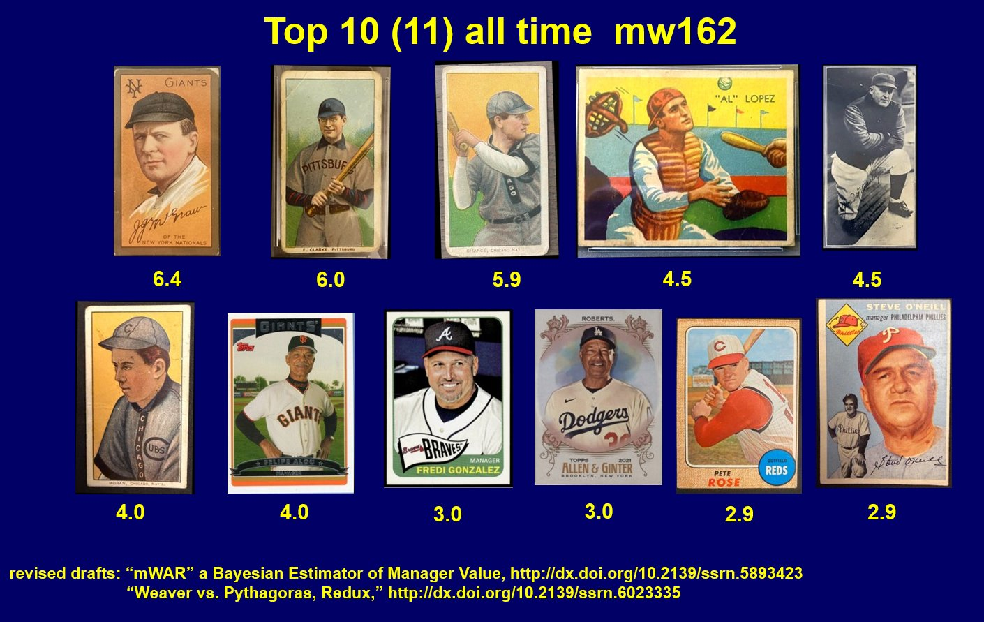
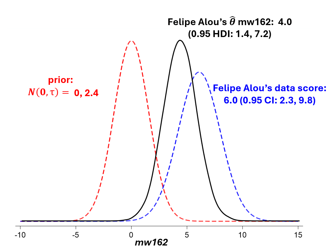
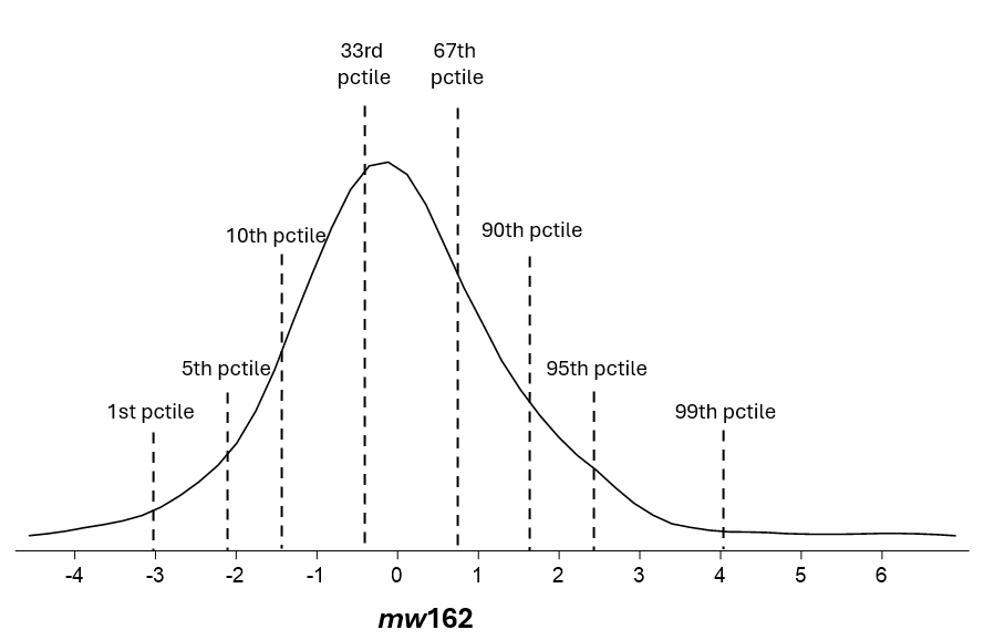
We can start with a prior of no manager effect in wins per season (162 games), with a standard deviation equivalent to observed manager heterogeneity. Then we take the benchmark player WAR model estimate of manager impact—6.0 wins per 162 games in the case of Felipe Alou. That’s the observed “data.” We then combine that data with our prior under Bayes’s theorem and come up with a posterior probability distribution, the modal value of which in Alou’s case is 4 wins per 162 games. That’s or most likely Bayesian mWAR value for Alou.
If we look at all the managers mw162 scores, let’s call them, the explain about 24% of the variance in team records that persists after we take account of team player WAR.
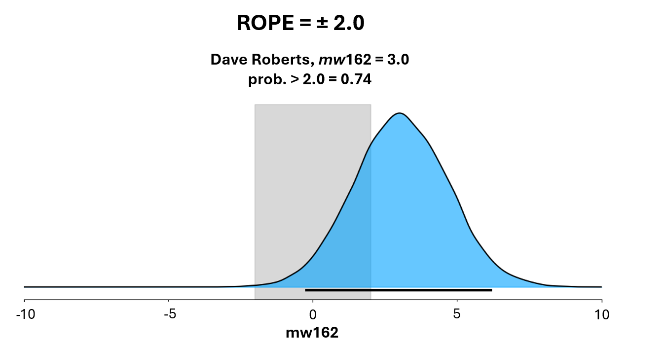
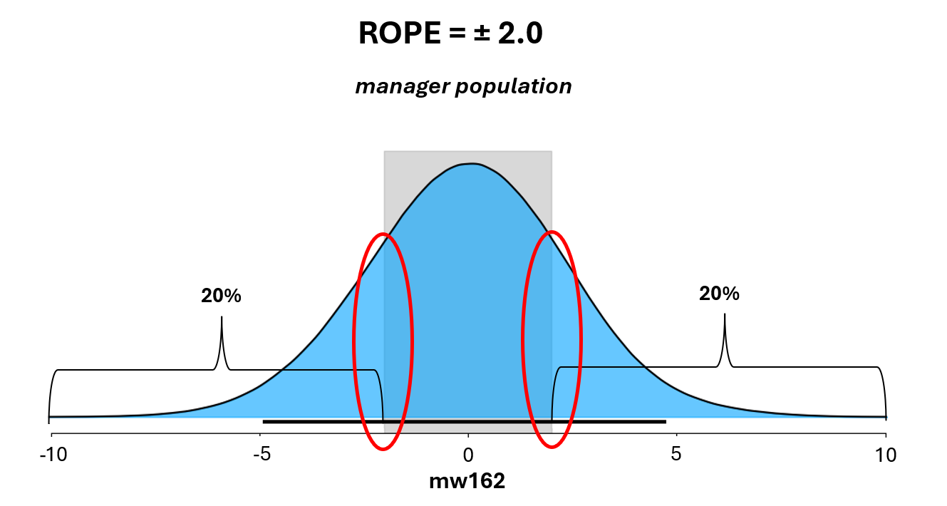
At that point, we can estimate the value of individual managers. One way to do so is by using a “Region of Practical Effect” or ROPE: we define cutoff beyond which we say that the manager impact will be viewed as practically important and see what managers’ posterior probability of exceeding that impact threshold is.
Let’s pick a rope of +/- 2 wins per 162 games (ignore the 0.02—that’s an optical illusion in my slide show). Bobby Cox has a mw162 of 2.3. The fraction of his posterior mass that exceeds 2.0 is 57%, which is our level of certainty or belief that he has an mw162 at least that high.
Dave Roberts has an mw162 of 3.0—and a 74% probability of >2.
 Tony LaRussa 2.4, 62%.
Earl Weaver, it turns out, is estimated to have an impact close to zero—or monkey level. Same for Billy Martin.
Lou Pinella is an example of a manager who is estimated to have cost his team 2 wins per season.
Another thing we can do customize the mWAR estimator to a users’ own personal utility function.
One reason to do that is the discrepancy between the estimator’s level of certainty about value of individual managers and its level of certainty about value across the manager population. Every year the Estimator learns about 30 times as much about managers as a whole as it does about any one manager. Accordingly, it can generate more confident estimates about what the prevalence of a particular level of skill in the population with much more confidence than it can about the level of skill of particular individuals.
If you look at individual estimates, it turns out that less than 10% of managers have an mw162 of +2—and about as few one of -2. But this individual-level assessment understates the frequency of this level of impact.
At the population level, the mWAR estimator estimates that about 40% of managers have mw162s outside the ± 2 threshold—half below, half above. That means there is a rich vein of talent, and a deep chasm of ineptitude, at these thresholds, consisting of managers who cannot be confidently identified.
So what should one do in this situation? The answer is engage in rational gambling.
Baseball economics are characterized by a tournament payoff structure. Teams that hit a certain level of wins get a super premium in returns in the form of post-season revenue.
Industries chracaterized by tournament payoff structures tend to foster distinctive risk preferences. Basically, particpants are risk preferring with respect to gains that can launch them over the super-premium threshold and risk averse with respect to losses that can drag them below it.
When it comes to hiring and firing managers, teams should be much more averse to underestimating than overestimating the skill of a potentially good manager. If he is one of the ones who can generate 2 or more extra wins a season, it could be a disaster to let him go; if he turns out not to be that good, then most likely his simply average, which is the most likely value of his replacement anyway.
By the same token, teams should be very averse to overestimating rather than underestinatintg the ineptitude of a potentially poor manager. If he is in the class that costs 2 games a season, holding onto him could wreck the team financially; if it turns out he wasn’t that bad, then his most likely was simply average, which is exactly the likely value of his replacement.
The estimator can be tuned to reflect exactly these risk preferences. This is relationship between the estimator assessment of a manager and his mw162 when over- and underestimating a manager are symmetric. But now imagine that teams have the asymmetric risk preferences described: they are twice as averse to mistakenly rating a manager with a skill level above 2 wins per 162 as below that level as they are to mistakenly rating one with a skill level below that threshold as being above it; and by the same token, the are twice as unhappy about rating a manger manger with a skill level below 2 losses per 162 as above that threshold as they are to mistkanely rating a manager above that threshold as below it.
When this loss function is fed into the Estimator, it the available posterior probabilities of all the managers to re-estimates their mw162s in a manner that maximizes the user’s utility. Here the observations in red are the sampled managers who are moved in one direction or another with respect to the +2 and -2 thresholds.
But this is only an example, the Estimator can be customized to fit any decision theory loss function a user chooses.
It is often said that the advent of sports analytics has rendered managers essentially irrelevant. But this in fact gets things upside down. Managers are consequential, and by using data appropriately, teams can maximize the contributions that they make to their success.