1.9.26 update: It’s monkey poop after all. Additional analyses, using more extensive data, a better model, and a superior strategy for forming a simulated empirical null confirm, as far as I can tell!, that there is no genuine manager influence detectable against the PE baseline. The reason is almost certainly that Horowitz’s critics were right: the PE formula defines an analytic speed-of-light limit that no manager (or team) can outrace. That doesn’t mean managers have no impact; it means only that the PE baseline is not a valid basis for determining whether this is so. Kind of sad that I was wrong but happy to admit it (mistakes are the engine of progress in knowledge–if you are willing to recognize when you make them).
So last time, we were on the verge of concluding that our featured managers’ Horowitz PHs were just a pile of monkey poop. The Monte Carlo Monkeys Playing Strat-o-matic (MC-MPS) simulation had created an apparent hierarchy of “skillful” and “inept” managers that had the same basic spread as the one we observe among real-world managers. So whatever we are seeing in the latter was, it seemed, indistinguishable from what we’d see on a planet of the monkey manager apes.
But it turns out, we didn’t really get what game those clever little primates were playing. . . .
Statistically speaking, we approached the monkeys as if they were a bunch of frequentists. That is, we tried to learn something from their games as if the issue of principal interest for them and for us was how many managers had Horowitz PHs ≠ 0 at p < 0.05. “Gee, 9 did. . . . But there that many in the MC-MPS, too. . . . And the probability of observing that number in either by chance was like 25%. . . . Meh.”
But as I said off-handedly last time, the monkeys had created a picture of random managing that’s actually a lot more informative and inference rich than a tunnel-vision frequentist outlook permits us to see.
The frequentist perspective appraises the relationship between the observed PH values and a normal distribution.
But the idea that PH values in the wild are normally distributed is just an assumption. They might not be. And that would affect our inferences about what the data show. If only we could see that real random PH distribution!
Well, the monkeys have taken care of that for us. Their game-playing reproduce the random process that generates PH inputs: runs scored and against at game level, consistent with manager-specific means and SDs), and corresponding wins and losses, aggregated at season level, for each manager. As long as we are confident that MC-MPS is faithfully capturing that process, then the monkeys’ hundreds of millions of games, comprising 131,000 manager careers, show us what real PH random distribution looks like!
Those crafty little cousins of ours what is known as an “empirical null” distribution. We should look at how our observed data lines up against that distribution—not a the theoretical, all-is-normal frequentist one. If real-world values fit snugly within or on top of that empirical null, then the monkeys have shown us that they should be hired immediately to skipper every MLB club. But if values at the tails of the real-world distribution poke out beyond those of the empirical null (do monkeys have tails?), then maybe Earl Weaver’s not just a monkey’s uncle after all!
Well, take a look:
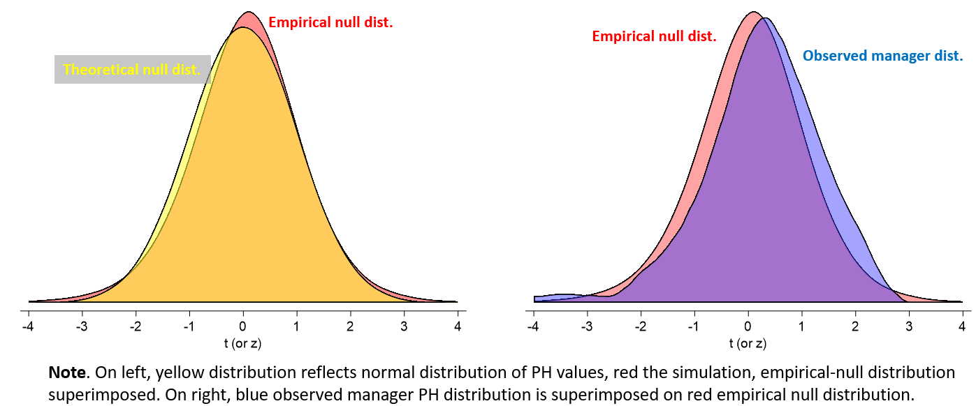
Actually, the empirical null distribution—the spread of PHs that the monkey managers compiled—is actually wider than a normal null distribution. That means that it is likely to generate a higher number of extreme, tail-end PH values than you’d expect to see if you assumed those values were normally distributed. Actually, if you wanted to think about this in frequentist terms, you’d treat p = 0.05 in the real manager data as only = 0.07.
But the real-world distribution is even more sprawling than that. We want to zoom in on those “enriched” tails—the ones that extend beyond the edge (particularly the right-side one) of the MC-MPS empirical null. What do data there tell us about the probability that our real-world managers have PH values that are truly ≠ 1. The empirical null actually (magically?!) gives us everything we need—prior odds, likelihoods, and posterior odds—to make a Bayesian estimate of the truth of the hypothesis that manager’s in that region have PH ≠ 1.0.
For that we are going to use another Bayesian statistical technique, called ROPE. That stands for Region of Practical Equivalence. To start, we specify some interval around PH = 1.0 in which we stipulate that the values are 1.0 “equivalent”; any value within that range fits comfortably within the distribution we’d associate with skill-free monkey managers’ PHs. Next we see whether the distribution of estimated PH values for any real-life manager falls within or outside that band: if inside, meh; if outside—hmmmm!
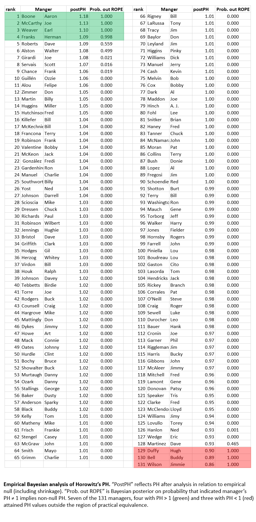
Let’s use a ROPE of PH 0.95 < PH > 1.08. Remember, Horowitz’s PH is an odds multiplier. It purports to tells how much more (or less) likely than even money (1:1) a manager is to win a game when his team generally allows as many runs as it scores. By selecting a ROPE of PH 0.95 < PH > 1.08, we are saying that we’ll recognize a particular manager’s PH ≠ 1 as a true indicator of his ability to influence game outcomes only when it implies that his personal decisionmaking would propel a .500 team to a record of .520 or better—or doom his player to a record of .490 or less.
Anything in between remains a “null” or “who cares?”
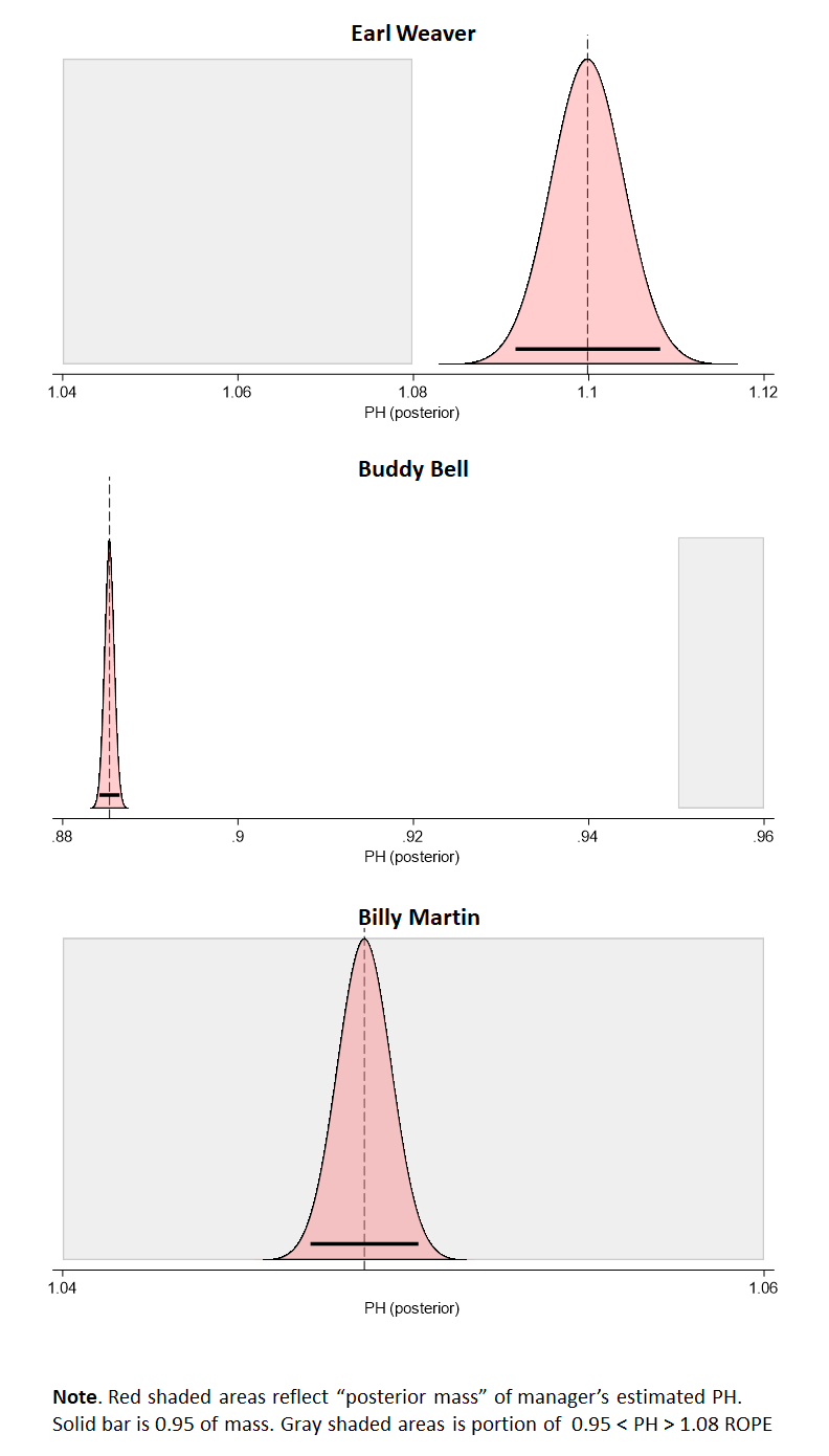
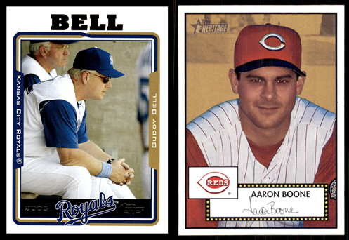
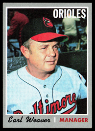
Basically, yeah, Earl Weaver is the real deal. His empirical-null adjusted PH is 1.10 (effectively, an expected winning percentage of .524 when he manages an expected break-even team). We don’t look only at the observed value; we treat the range of values around 1.11 as his PH, because there is imprecision in our measuring instrument. But the resulting “density mass” of values is so far beyond 1.08 that his Bayesian posterior probability for PH ≠ 1 is essentially 100%.
 Buddy Bell (happy birthday!) is a true PH ≠ 1, too. But it points in the opposite direction. The mass of values we treat as his possible range, which is densest as PH = 0.88 and change, falls far, far short of the 0.95 boundary we decided to treat as equivalent to a monkey-manager PH = 1.0
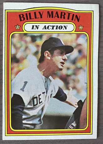
And finally, Billy Martin. His observed PH was about 1.05. But that doesn’t cut it. We don’t think this outcome, which implies a .510 record when Billy manages a .500 team, is genuinely indistinguishable from one we might have seen with a monkey rolling dice.
Now all of this is with my ROPE set at 0.95 < PH > 1.08. If your “meh” zone is wider or tighter—adjust it, and see what the revised posteriors for true PH ≠ 1 turn out to be! Cool!
Now, one more thing. . . .
Is Aaron Boone the best manager ever? He has the highest empirical-null adjusted PH: 1.17—an expected .539 win pct for a .500 club! But does that really mean he is better than Earl Weaver?
We can also use the insight gained from our empirical, monkey-manager null to address this question. We can set another ROPE, this time for a zone of equivalence in which we say about Boone’s edge, “meh, that’s really not meaningfully different from Weaver’s PH.” Let’s pick a ROPE that supports the Boone-better-than-Weaver hypothesis only if Boone’s PH is at least 5% higher than Weaver’s.
Here’s what we get:
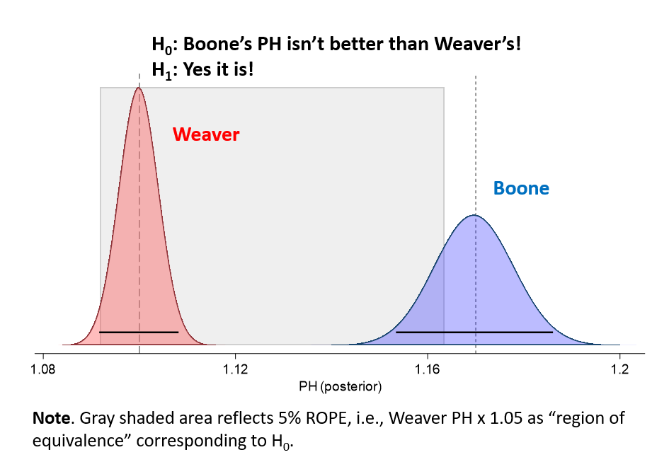
It’s a closer call than whether either of them has a true PH > 1.0. Boone’s “posterior mass”—the estimate of the range and density of values associated with our best measurement of his PH—doesn’t fully fall outside the ROPE. But enough of it does so that our Bayesian posterior is that there is a 94% chance Boone would do better when he manages a .500 club than Weaver would.
Do you believe that?
 The answer still depends on what you think of Horowitz’s PH.
Don’t decide whether it’s valid based on whether you like the results—that’s confirmation bias. Instead try to decide on the basis of validity-relevant evidence independent of your prior beliefs.
These last two posts try to furnish you with evidence of that sort. Now you have to decide, using your own powers of critical assessment, what you think of it!
One last point on this: even if you find everything presented here compelling, all I’ve really done is furnish reason to believe that Horowitz’s PH is measuring something real; that it’s not—as Horowitz’s critics maintained—just noise; that, in other words, it’s not just a report card on how well monkey managers did playing Strat-o-Matic!
But I haven’t done anything to show that what it is measuring is really manager skill. That would take evidence of an entirely different sort.
These two types of validity are often called “internal” and “external”: the former relates to whether an estimator is genuinely producing accurate and valid measurements; and the latter to whether what’s being measured is what the thing in the world that the estimator is supposed to be estimating.
Is Horowitz’s PH externally valid? I’m really not sure.
What do you think? And do you have any ideas on what sorts of empirical tests would help us figure that out?! The monkeys are all ears!